Hawk Eye

Automatic Birds Eye View Registration of Sports Videos

Abstract:

The sports broadcasting viewing experience has essentially remained unchanged for decades. A camera position on the side of the playing field which pans according to where the focus of the game is at that moment. However, with current technology and computer vision, we can overhaul this viewing experience from a purely 2D perspective and closer to a 3D experience which includes the side and top view. We do this by creating a dictionary of corresponding edge maps which have been obtained by transforming the side view to the top view with homography matrices. When a new image is obtained, we transform into an edge map using Pix2Pix and then retrieve the closest matching edge map(and its corresponding homography) from the dictionary. We obtain a mean IoU score of 0.833 on the test dataset. We also obtain fairly good results on broadcasting identified players into the top view.

Introduction:

Tactics and strategies for sports are largely depicted on the top-view of game field. For a lot of sport analytics to happen, we need to convert the camera view broadcast stream to a top view that helps understand player movements in-game. This is typically achieved with an expensive multi-camera set up around the field. The views from these cameras are then annotated by hand and converted into a top view. This limits the use to only those that can happen after a match has been broadcast. However, if this process is automated, it would open up multiple avenues of analytics and sports viewing that can occur concurrently with the match that is currently being broadcasted. We use Computer Vision techniques to solve this problem in a semi-supervised manner. We test our method specifically for soccer data but it can be adapted to similar sports like basketball and hockey. We generate homographies between images from particular camera views to the corresponding location in the top view field (which will be in the form of an edge map representing a football field) and create a large database of such edge maps along with homography matrices using camera perturbations. During test time, we use a pix2pix deep network trained on our database obtained in this way to obtain corresponding edge map. This is queried through the database to get a homography matrix which obtains a top view of that test image. Furthermore, we identify the player in each camera view by subtracting green field and doing template matching on the contours present in the image. The identified players can then be broadcast into the top view and appear as points which can be tracked. In this way, we can obtain relevant statistics from just the broadcast video stream of the match via an efficient solution that does not require any expensive camera setup.

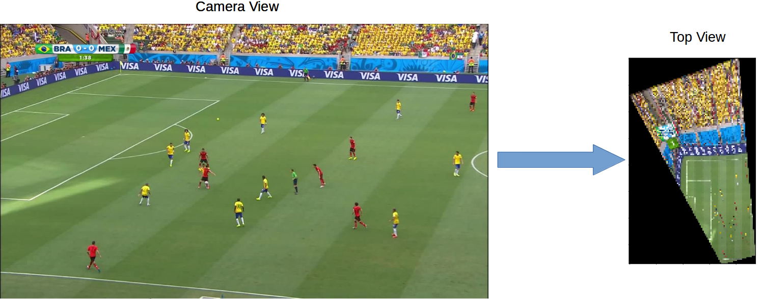Camera View to Top View

Approach:

1. Edge Map Generation:

The dataset we are using is the World Cup dataset collected by http://www.cs.toronto.edu/~namdar/pdfs/sports_cvpr_2017.pdf. The dataset consists of frames of 20 different soccer matches played during the 2014 World Cup. The 210 frames in the training dataset and 200 frames in the test dataset, each having a homography matrix, is used to map the camera view into the top view. We create an edge map of a top view as a reference image for the homography transformation.
First we annotate all 210 frames with 4 point correspondences from the actual camera view image to the top-view projection blueprint. Using these 4 correspondences we generate the homography matrix for these annotated images and their corresponding top-view. We use the blueprint to get the edge map using the inverse homography matrix.
We apply this method to all 210 frames in the training dataset and the generated edge map is placed in the dictionary along with the corresponding homography matrix that was used. This forms the base of our dictionary which we augment further.

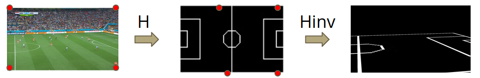Using inverse homographies to generate edge maps.

2. Augmented the Dictionary:

The current dictionary of 210 frames will be insufficient for querying during test time. So we augment the database by virtually changing the camera position of the training images and then generating the edge map and corresponding homography matrix that is obtained. We perturb the camera position through three methods, namely panning, tilting and zooming. We obtain the 4 correspondences of the quadrilateral($q_0, q_1, q_2, q_3$) in the camera view and the top view and then transform these coordinates using the equations associated with each type of perturbation. The transformation is done first in the top view. The values used for each perturbation were selected after analyzing which gave the best results.

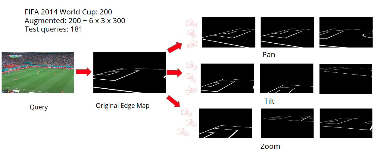Generating augmented data by adding basic perturbations.

Pan: We simulate pan by rotating the quadrilateral $(q_0q_1q_2q_3)$ around the point of convergence of lines $(q_0q_3)$ and $(q_1q_2)$ to obtain the modified quadrilateral. Values used for pan were [-0.1, 0.1, 0.15, -0.15, -0.18, 0.18].

Tilt: We simulate zoom by applying a scaling matrix to the homogenous coordinates of $q_0, q_1, q_2 and q_3$. Values used for tilting were [-0.05, 0.05, 0.02, -0.02, -0.035, 0.035].

Zoom: We simulate tilt by moving the points $q_0, q_1, q_2, q_3$ up/down by a constant distance along their respective lines $(q_0q_3)$ and $(q_1q_2)$. Values used for zooming were [0.95, 1.1, 1.2, 1.15, 0.9, 0.85].

We apply the perturbations to each of the images with 6 different values for each perturbation. This results in 18 output edge maps for each input frame in the training datasets. We create new homographies for the perturbed trapeziums in the top view to rectangular images of the original camera view. We then store the edge maps obtained by transforming into the camera view and the associated inverse of the homography matrix that was generated earlier into the dictionary. This increases the dictionary size from 210 to 3980. This dictionary now gives a larger chance to find matching images which are identical or nearly identical to the query input.

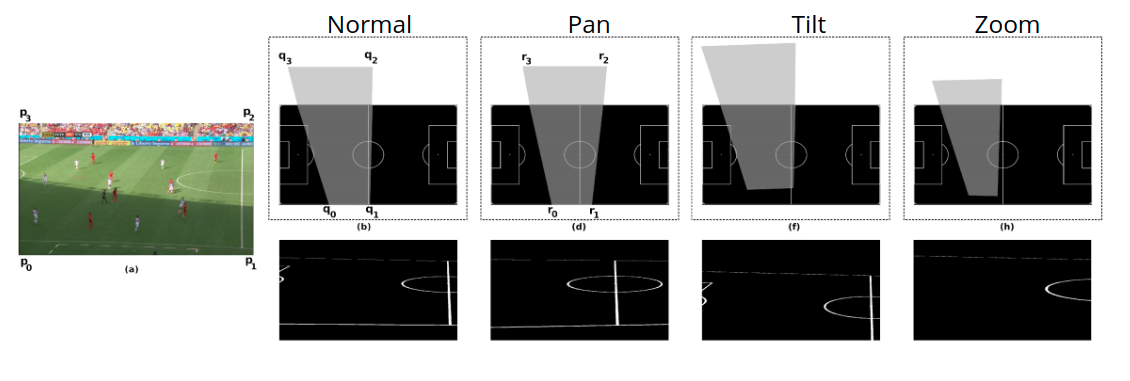Samples of augmented images generated using pan, tilt and zoom transformations.

3. Pix2Pix Training:

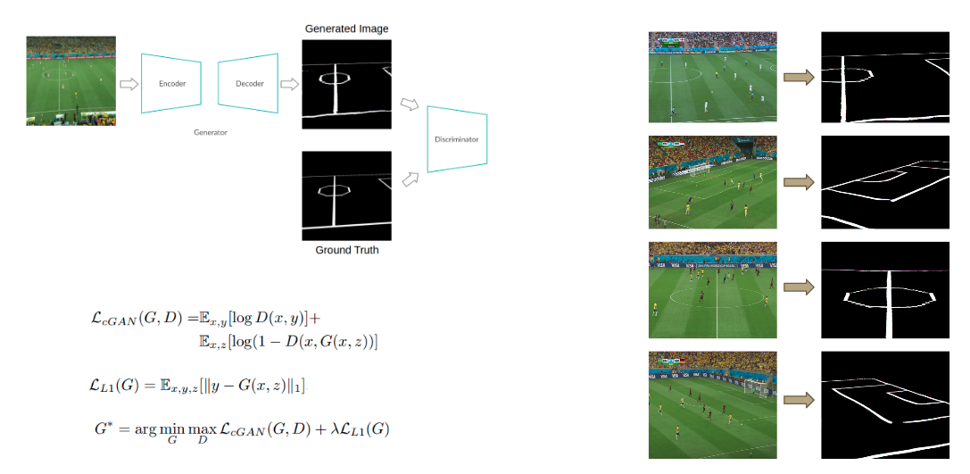
During test time, we convert the camera view frame input, into its equivalent edge map so that it can be queried with our dictionary. To do so we need to use image-to-image generation which is why we picked the pix2pix model. We use pix2pix to generate edge maps from camera images.

Samples of augmented images generated using pan, tilt and zoom transformations.

Pix2pix is a conditional generative adversarial network which translates an input image $x$ from Domain 1 into its corresponding image in Domain 2. Domain 1 will be the camera views from the training dataset. We generate the edge map for these images by using the inverse homography by using the inverse of the associated homography matrix with top view edge map as the source image. The generated edge maps form Domain 2 for the training process. We then trained pix2pix to learn a mapping from Domain 1 to Domain 2. During testing, we convert the input image from camera view to an edge map using the trained pix2pix model.

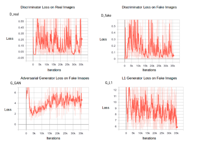Pix2Pix Training Loss Curves

4. Matching and Retrieval of H*

With the dictionary complete and the pix2pix model completely trained, we can input an unseen frame from the test dataset and retrieve back the closest edge maps. Histogram of gradients (HoG) is applied on all edge maps in the dictionary, and using the HoG, a KNN model is trained and used for querying. We only use the closest match (i.e. nearest neighbour) to find the homography for the query image. The entire pipeline for querying will be :

1. First the query frame is input to the pix2pix model. This will return an edge map of the same image in the camera view.
2. The generated edge map is used as a query to the dictionary that was created. Based on the HoG value of the generated edge map, it is matched to the closest neighbour in the generated KNN space.
3. With the closest edge map identified, the associated homography matrix is also returned, which can be used for projecting the query image into the top view.

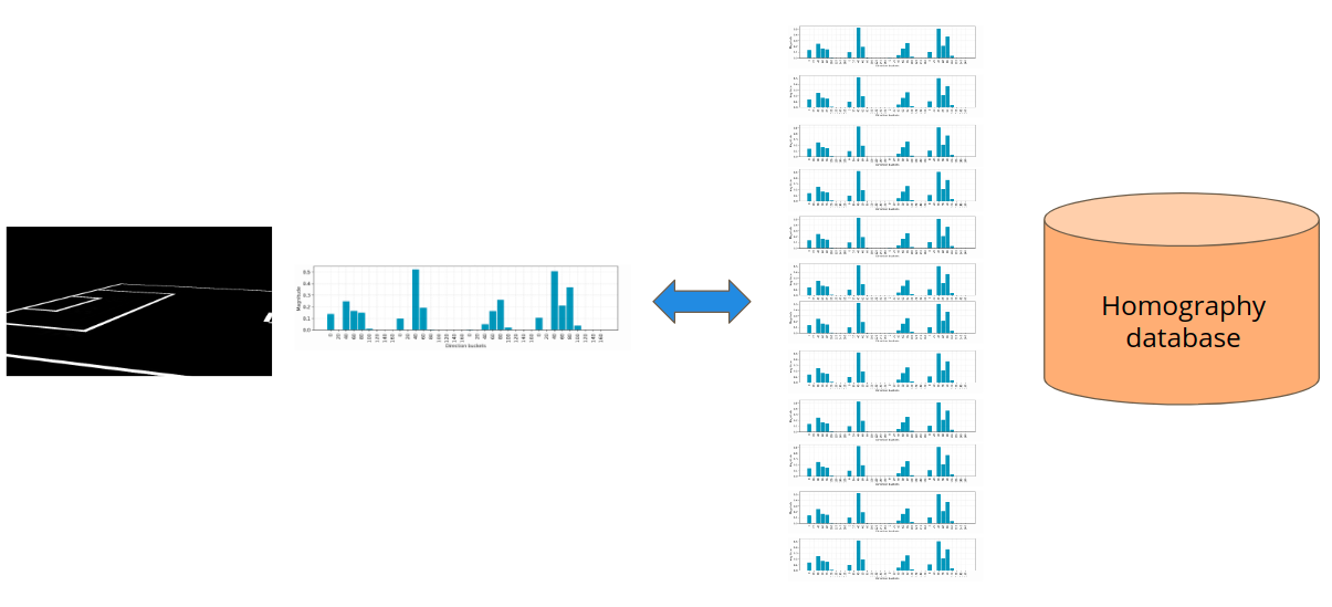KNN matching to find associated homography of closest matching edge map

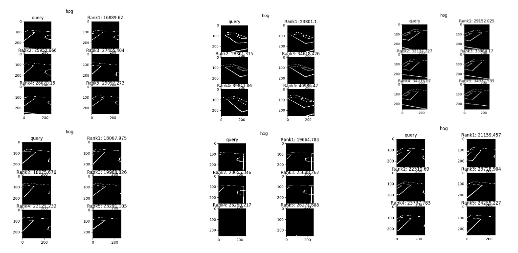KNN matches with K=5 for some samples

5. Projection onto top view with H*

With the best homography matrix for the query image identified, we can transform the camera view into the closest approximation of its corresponding top view edge map. The transformation can be applied on either the generated edge map or the actual camera view image. For player mapping we use the camera view with the identified players annotated and mark the players as circles in the top view.

6. Player Mapping

Player mapping is done in two steps. The players first have to be identified in the camera view. This is done by first identifying the field in the soccer image by identifying all the green pixels in a particular range. The identified pixels are used as a mask for the field which is then separated from the remaining part of the image, leaving only the players and part of the background. We do morphological closing operations on the filtered image, which will fill out the noise that is present in the crowd. This reduces the possibility of false detections. After this process, we check for contours in the image. For each detected contour, we check if the height is more than the width (at least 1.5 times) which will be our detected players. We resized each detected sub-image of a player to 30x30 pixels and applied K-Means with 2 clusters on all these sub-images. The 2 most detected pixel colours will be the colors of the teams’ jerseys. For each sub-image we search for these two pixel colours and then assign the player to the colour that was dominant. With the player and team identified, they can be mapped to the top view accurately.

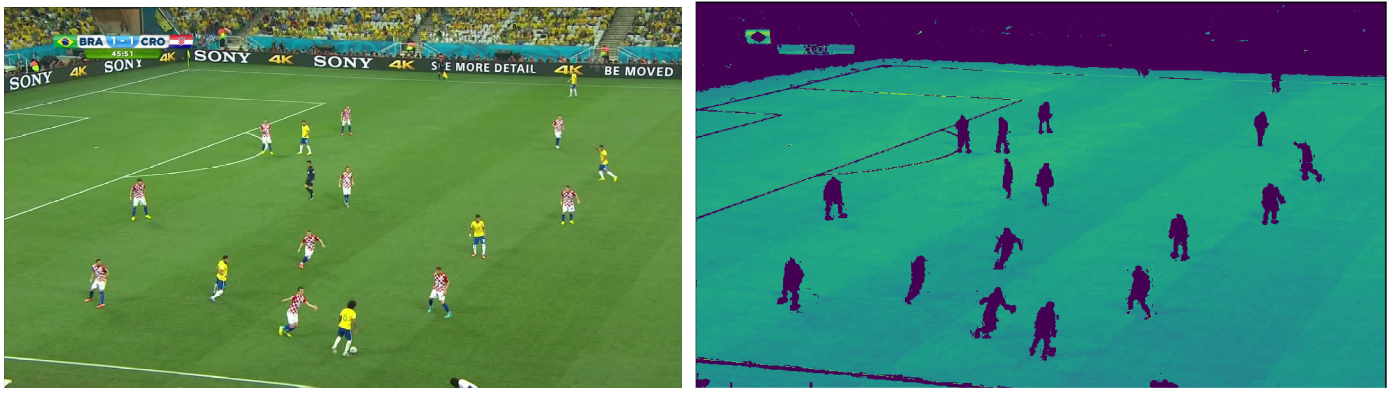Input Image and filtered image to mask out players

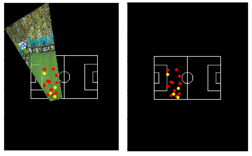Top View Projection with players

Experiments and Results

We create a test-train split on our initial dataset. Using our augmentation technique, we build a reasonably large dictionary and find the homographies for the test images. To measure the accuracy of our results, we compute an Intersection over Union score as described below. We also present a qualitative analysis where we superimpose the top view projection of the camera image onto the football field and visually compare the results.

Quantitative results

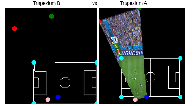
Based on the actual ground truth homography in the dataset, the camera view image is transformed into a trapezium in the top view space (trapezium A). Similarly, the predicted homography by our system, using the closest match from the trapezium projects the camera image into another trapezium (trapezium B). We clip the two trapeziums with the football field to get the area that we are concerned with (i.e. only the area covered in the football field).

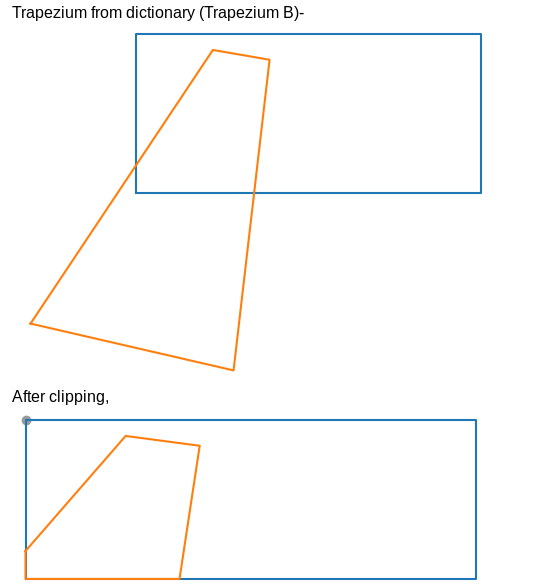
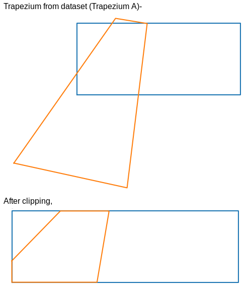
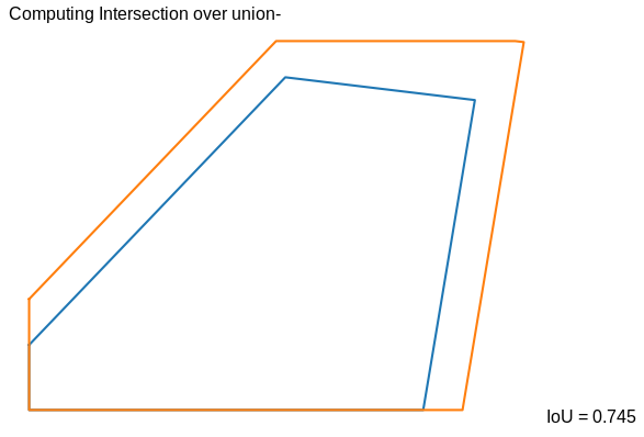
We obtain a mean IoU score of 0.833 on the test set using this approach.

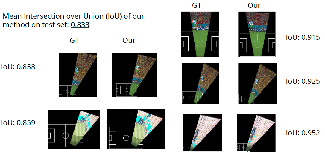
Qualitative results

Qualitatively, we can compare the top view projections using the Ground Truth homography and the homography predicted from our system. Doing this we can confirm the results are reasonable.

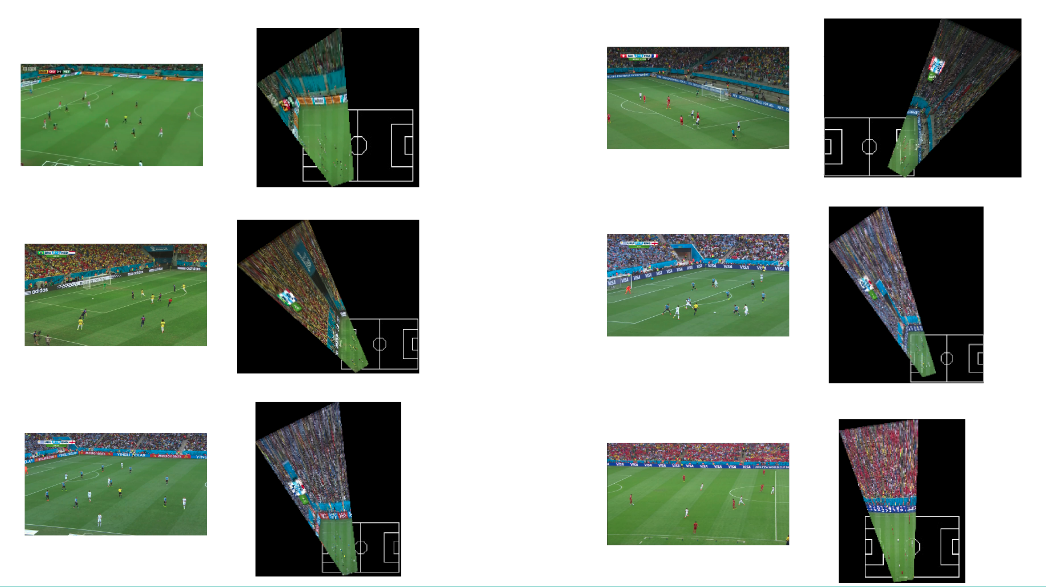
Here are a few more results with the camera input against the top view generated by our system-

Conclusion and future work

We successfully generated a top view for a given camera view of a soccer game. We also successfully achieved our stretch goals of doing player detection and mapping. With the camera view being mapped to a top view automatically, it removes the need to do this by hand and will greatly speed up sports analytics and can have a transformative experience on the sports broadcast experience which has remained static for decades. We have only established the basic foundation for this and believe that more can be built on this work.

Using deep networks with contrastive or triplet loss with hard negative mining would improve the reliability of the querying results and improve results on multiple weather conditions and different types of fields. Allowing a user to view both the camera and top view for a live broadcast would allow for a more complete and complex analysis for teams and an enriched experience for viewers. Player mapping is currently unreliable and prone to losing players between frames. This can be improved by estimating their trajectory via optical flow and tracking techniques (like Kalman filter based) for frames where they are not correctly identified and make the model more robust. As a whole, the entire dictionary can also be made much larger and with more camera transformations since the performance of our method can scale with increase in the amount of data. This would improve the IoU score as there is a higher probability that there is a match in the query database.

References:

https://faculty.iiit.ac.in/~vgandhi/papers/sbgj_wacv_2018.pdf
http://openaccess.thecvf.com/content_CVPRW_2019/papers/CVSports/Chen_Sports_Camera_Calibration_via_Synthetic_Data_CVPRW_2019_paper.pdf
http://www.cs.toronto.edu/~namdar/pdfs/sports_cvpr_2017.pdf
https://www.cs.ubc.ca/~murphyk/Papers/weilwun-pami12.pdf
http://web.engr.oregonstate.edu/~afern/papers/register-cvpr07.pdf
https://www.cs.ubc.ca/~lowe/papers/okuma04b.pdf