Motivation
Football is among the most popular games in the world, with more than 80 leagues played across the world. The English Premier League is one of the most ferociously contested leagues in the world, and of late, has also made the fans of the game competitive too. Applications like the Fantasy Premier League, have come up which requires fans to make teams for each gameweek by predicting which players are going to do well.
At the onset of the project our intent was to develop a framework that aims to predict the performance of each player in a game given the past performance metrics over several matches. Using a dataset[1] of English Premier League matches over four seasons that have certain player statistics for each game, we intended to train a LSTM based sequence model to predict their performance in an upcoming match (a single numeric rating) given the performance of every player in the team over the last matches.
In addition, we want to use an unsupervised learning based clustering approach to group players by position and skill.
The predictions of our supervised learning framework, which would return players with their predicted ratings for the next match, can help players of Fantasy Premier League, in deciding which players to have in their teams for the upcoming gameweek, in a a way that will maximize their points.
Dataset
Our dataset[1] contains the data of 20 Premier League teams, over four seasons (2014-15, 2015-16, 2016-17,2017-18). Each year contains data for the 20 Premier League teams, and the results and statistics of all matches that took place in the league in the respective year.
There are 31 features that we have for each player- ‘aerial_won’, ‘blocked_scoring_att’, ‘error_lead_to_goal’, ‘saves’, ‘att_pen_post’, ‘penalty_save’, ‘post_scoring_att’, ‘goals’, ‘total_pass’, ‘clearance_off_line’, ‘accurate_pass’, ‘good_high_claim’, ‘att_pen_goal’, ‘att_pen_target’, ‘six_yard_block’, ‘red_card’, ‘goal_assist’, ‘second_yellow’, ‘fouls’, ‘total_tackle’, ‘won_contest’, ‘yellow_card’, ‘att_pen_miss’, ‘last_man_tackle’, ‘own_goals’, ‘total_scoring_att’, ‘touches’, ‘penalty_conceded’, ‘aerial_lost’, ‘formation_place’, ‘man_of_the_match’.
Feature Engineering
For each team, only the 11 players who have played a particular match have non zero attributes for that particular match. We disregard substitutes to avoid any skew in statistics to creep in. For each player we select only 13 of the 31 features.
| Feature | Types | Description |
|---|---|---|
| aerial_won | float | percentage of aerials won |
| aerial_total | int | total aerial dues |
| accurate_pass | int | accurate passes made |
| total_pass | int | total passes attempted |
| total_tackle | int | total tackles made |
| won_contest | int | total contests won |
| goal_assist | int | number of assists |
| goals | int | number of goals scored |
| touches | int | total number of touches |
| man_of_the_match | boolean | man of the match |
| fouls | int | fouls committed |
| total_scoring_att | int | total scoring attribute |
| saves | int | total number of saves (for goalkeepers only) |
Supervised Learning
Task:
Find player ratings for the next match of Team A and Team B given player performance attributes over past 10 games of both the teams.
Input Representation:
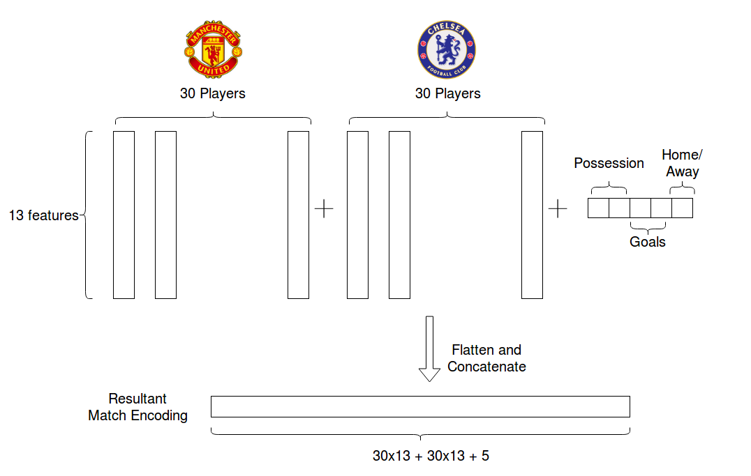
We have noticed that in all the seasons, the maximum number of players that a team has had during a season are 30. So for each match we take our input array as a (30x13) length array for each team, where 30 is the number of players and 13 are the features selected for each of these players.
We take these two (30x13) length matrices as input for our LSTM, along with 5 other features which include full time score, full time possession and a feature that depicts whether the game was home or away. This gives us the match encoding that we use later as input.
This forms our 30x13 + 30x13 + 5 input representation.
Architecture:
The architecture of our Supervised Learning framework is as follows:
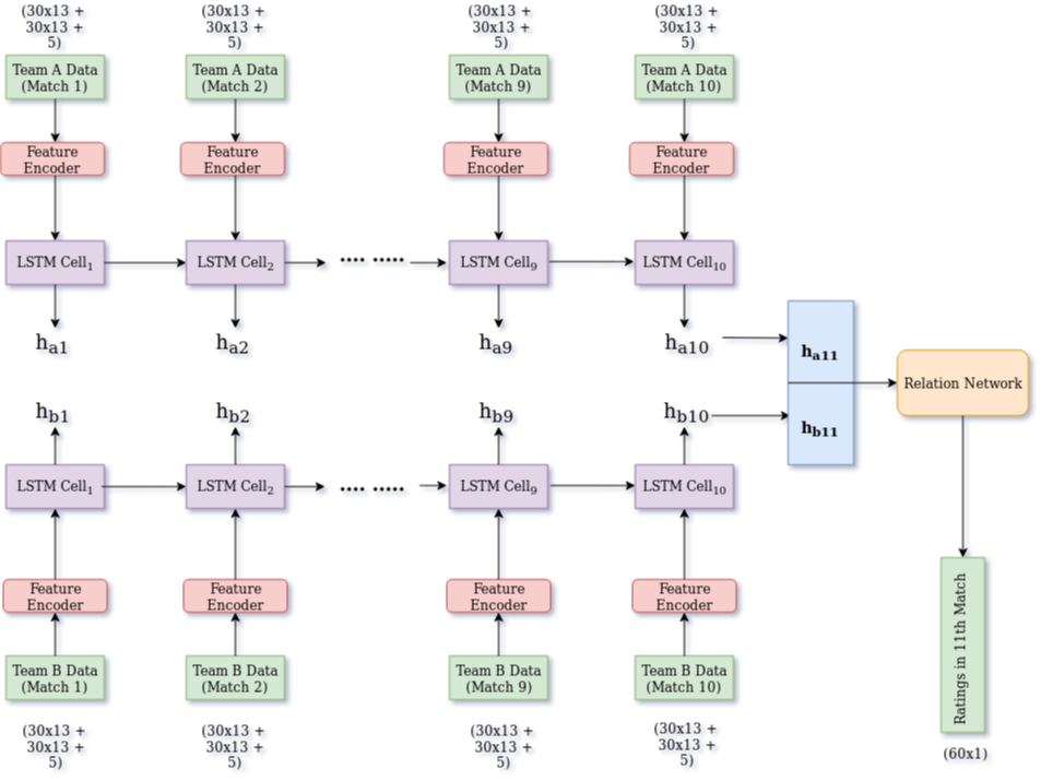
We create a match encoding from the player attributes and aggregate match statistics as described above. We use an embedding layer to create a denser representation that serves as input to the LSTM. The LSTM captures the information in the last 10 games for each team. The final hidden states of the two LSTMs are then concatenated to serve as a representation that captures the form of the players in both teams. A fully connected layer along with a sigmoid layer acts on top of this to finally find the ratings of all the players from both teams in the next match.
Why this approach?
We use an LSTM based sequence modeling approach because the data is temporal in nature, in that the recent results of a team and players carry more weightage than the older results. Thus we aim to capture the temporal information using an LSTM. Further, once we have extracted the form of both teams, we apply a fully connected linear layer so that we get the performance ratings of the players relative to each other.
Experiments and Results
-
Beginning with an input representation containing all the features (31) from the dataset, we prune the features we select. We find that only 13 of the 31 features are representative of the information that can be used to predict player ratings.
-
We also perform hyperparameter tuning. Below is a detailed ablation analysis-
| Method Used | Train MSE | Test MSE |
|---|---|---|
| Batch Size=32, Hidden Dim=16, Embedding Dim=32, Dropout=0.5 | 0.178 | 0.232 |
| Batch Size=16, Hidden Dim=16, Embedding Dim=32, Dropout=0.5 | 0.177 | 0.224 |
| Batch Size=8, Hidden Dim=16, Embedding Dim=32, Dropout=0.5 | 0.183 | 0.232 |
| Batch Size=4, Hidden Dim=16, Embedding Dim=32, Dropout=0.5 | 0.173 | 0.236 |
| Batch Size=16, Hidden Dim=32, Embedding Dim=32, Dropout=0.5 | 0.181 | 0.217 |
| Batch Size=16, Hidden Dim=64, Embedding Dim=32, Dropout=0.5 | 0.209 | 0.227 |
| Batch Size=16, Hidden Dim=32, Embedding Dim=16, Dropout=0.5 | 0.205 | 0.240 |
| Batch Size=16, Hidden Dim=32, Embedding Dim=64, Dropout=0.5 | 0.197 | 0.240 |
| Batch Size=16, Hidden Dim=32, Embedding Dim=32, Dropout=0.25 | 0.185 | 0.238 |
| Batch Size=16, Hidden Dim=32, Embedding Dim=32, Dropout=0.75 | 0.190 | 0.223 |
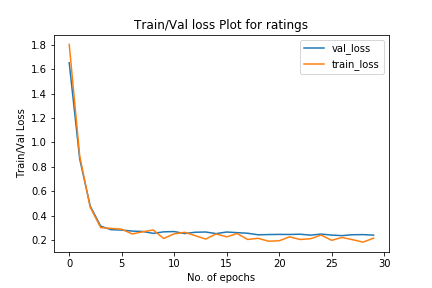
- Below is the training and validation loss curve for the best result above-
- In addition to the proposed task, we also perform the task of predicting the result of the next game, given past 10 performances for both teams. On this task we get an accuracy of 67% on our test set and a 98% accuracy on the training set, which is significantly better than a random classifier which would have a 33% accuracy (Win, Lose, Draw).
Discussion
We split our 4 seasons data into train (3 seasons) and test (1 season). With the best hyperparameters and the best feature selection, we get an MSE score of 0.217 on the test set. This translates to an average absolute error of 0.23 in the predicted player ratings as against the ground truth. We believe this is a good result since the player ratings vary between 0 to 10. This score can be further improved by using a larger corpus that has data from more seasons and more leagues.
Unsupervised Learning
Architecture:
The architecture of our Unsupervised Learning framework is as follows:
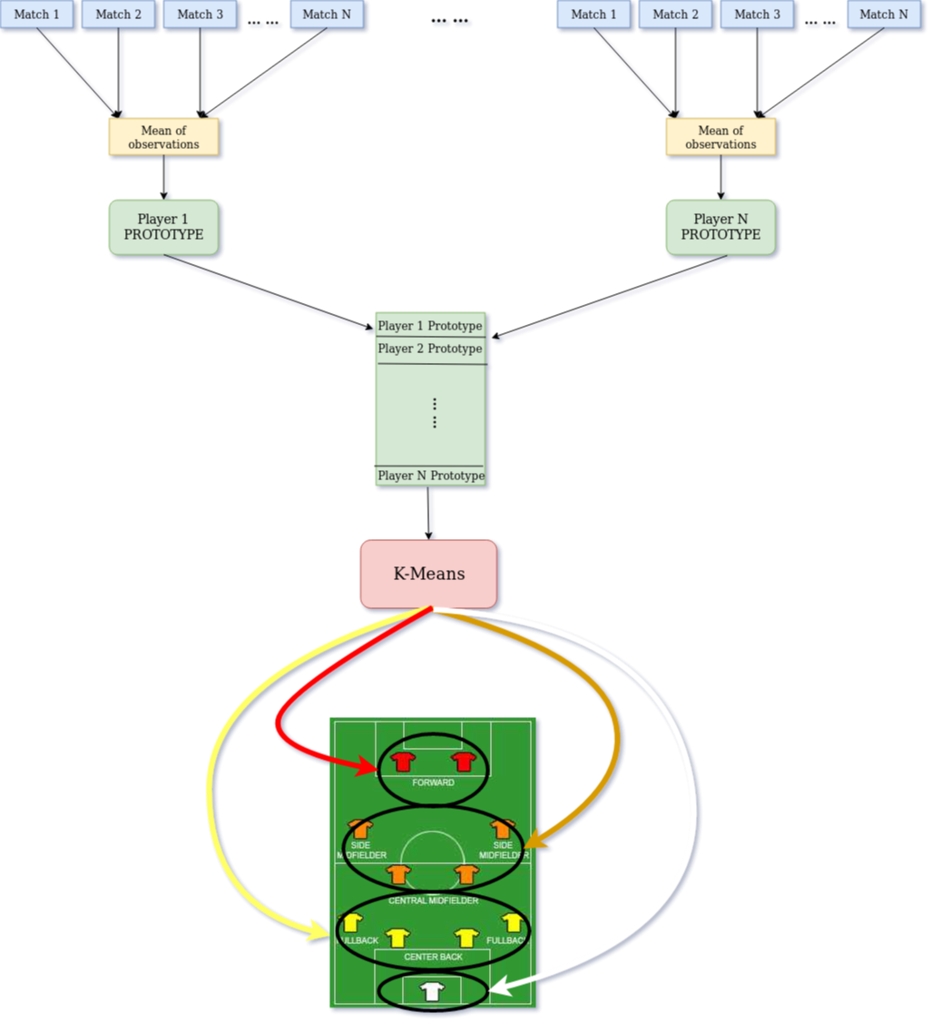
We compile the 13 feature components for each players into a player based dictionary. For each player, we construct a prototype which is the average of the normalized feature elements. On this set of prototype players, we want to group them into four clusters. This is because there are mainly 4 types of positions- Goalkeepers, Defenders, Midfielders and Attackers.
Why this approach?
For every player, we aim to find the average statistics over all games so as to weed out outlier performances. Since K-means and other clustering algorithms are sensitive to magnitude of features (as they compute distance between data points), we normalize the features so as to remove the impact of scale on features.
We wanted to try K-Means because this follows the approach that we want to divide the data into k sets and compare the data samples with each other. We tried Agglomerative clustering because the division is done in a sequential way where data is merged one at a time until k sets remain.
The reason we try doing dimensional reduction with PCA before applying the clustering algorithm because many of the data samples are sparse and we wanted to see if we could leverage this for better performance.
We use Purity, DB Index and Silhouette Score to evaluate the performance of the clustering methods on our data.
Experiments and Results
We experiment with both K-Means and Agglomerative Clustering and we also assess if performing dimensionality reduction with PCA helps the performing as several data samples are sparse. For PCA, we choose the number of components to be 4.
| Method Used | Purity | DB Index | Silhouette Score |
|---|---|---|---|
| K-Means (k=4) | 72.15 | 1.523 | 0.248 |
| PCA (k=4) and KMeans (k=4) | 73.04 | 1.104 | 0.347 |
| Agglomerative Clustering (k=4) | 65.89 | 1.688 | 0.1757 |
| PCA (k=4) and Agglomerative Clustering (k=4) | 76.25 | 1.2258 | 0.3292 |
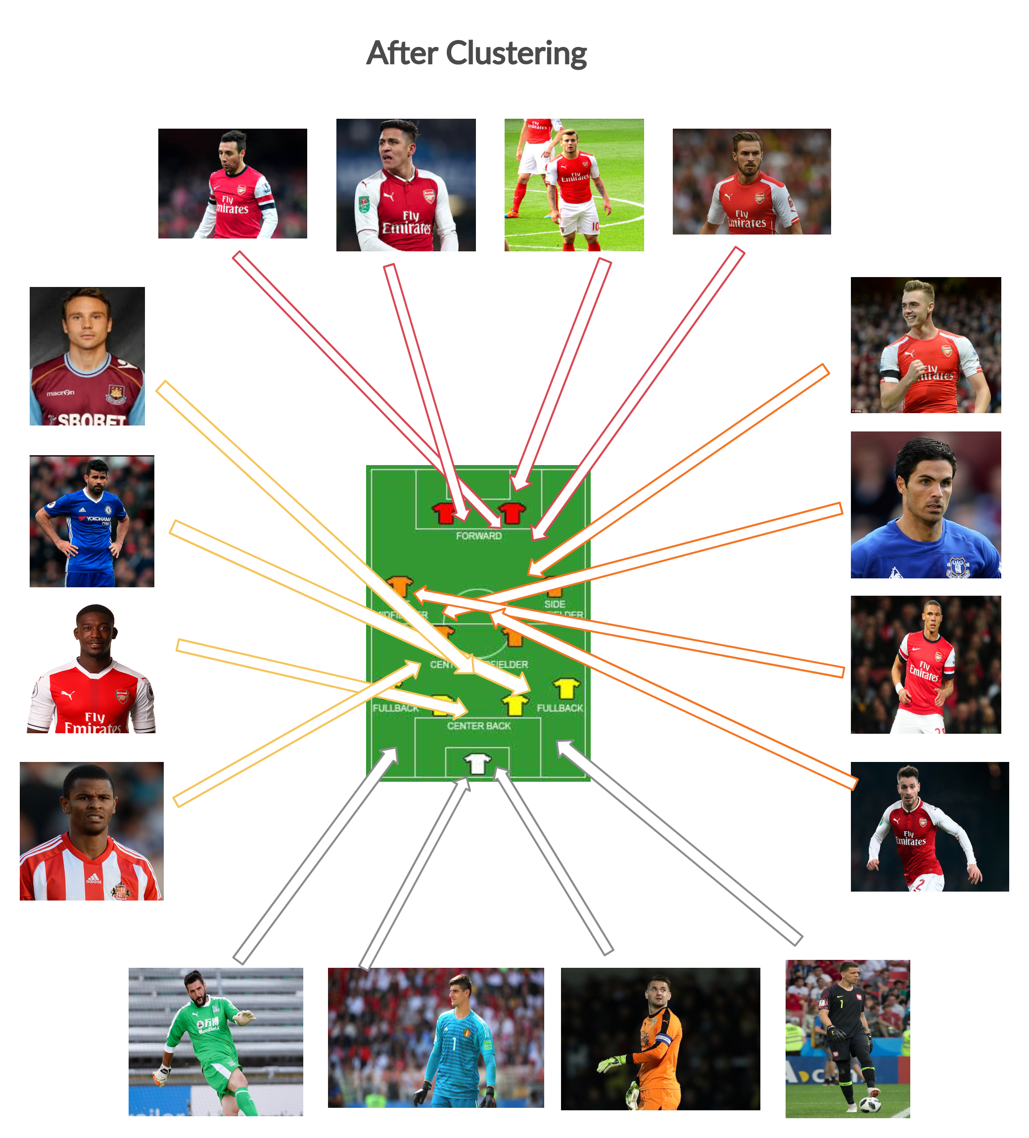
Discussion
We observe that PCA + Agglomerative obtains the best results even though just Agglomerative (basically the boost when doing PCA is more for Agglomerative over K-Means). We believe this is because Hierarchical clustering methods are able to leverage less sparse feature sets in a more discriminable manner. But in general, performing PCA seems to be improving the result for clustering.
Conclusion
We have successfully managed to train our supervised learning framework that is able to predict the player ratings for an upcoming match, with good accuracy. We have also been able to predict the outcome of the coming match with an accuracy of about 70% which is good, but can be reported in the future, if we have a large enough corpus to train our model with. We have also successfully managed to compare a host of unsupervised learning algorithms to predict player positions and have attained good results with the same.
References
- [1] Shubham Pawar. English premier league in-game match data https://www.kaggle.com/shubhmamp/english-premier-league-match-data, Mar 2019.
- [2] Geetanjali Tewari and Krishna Kartik Darsipudi. Predicting football match winner using the lstm model of recurrent neural networks, June 2018.
- [3] Sepp Hochreiter and Jürgen Schmidhuber. Long short-term memory. Neural computation, 9(8):1735–1780, 1997.
- [4] Daniel Pettersson and Robert Nyquist. Football match prediction using deep learning, 2017.